Implementing a Simple Neural Network

From theory to practice: let's build a neural network with PyTorch!

In the previous articles, we explored the fundamental concepts of neural networks and deep learning, understanding how these technologies work and why they are so powerful.

Now, it's time to put that knowledge into practice and build our own neural network from scratch! 🚀

We will use the PyTorch library to build and train a simple MLP (Multilayer Perceptron) neural network for handwritten digit classification using the MNIST dataset.

You can find the code on Colab at: https://exploringartificialintelligence.substack.com/p/notebooks

Setting Up the Environment

To follow this tutorial, you'll need Google Colab or an environment with Python and PyTorch installed.

Google Colab is a great option since it already comes with PyTorch support and allows the use of GPUs for free.

The MNIST Dataset

MNIST is a classic dataset consisting of images of handwritten digits (0 to 9) in grayscale, with a size of 28x28 pixels, where each digit has its corresponding class (0 to 9).

This dataset is widely used for experiments in pattern recognition and machine learning.

Let's code!

We are going to create a training and testing code for a neural network using the MNIST dataset, which contains images of handwritten digits. Let’s go step by step through what the code does.

The architecture we will use is a simple neural network, with a single fully connected layer that receives the images as input, "flattening" them into a 784-dimensional vector (28x28) and generating 10 outputs corresponding to the classes (digits 0 to 9).

The model will be trained with the CrossEntropyLoss loss function and the SGD optimizer.

Importing the necessary libraries:

• torch and torch.nn: Used to create and train neural networks in PyTorch.

• torch.optim: Provides optimization algorithms such as Stochastic Gradient Descent (SGD) used here.

• torchvision.datasets: Imports the MNIST dataset and other libraries for image manipulation.

• torchvision.transforms: Used to perform transformations on images, such as converting them to tensors.

• matplotlib.pyplot: Used to visualize the images.

import torch
import torch.nn as nn
import torch.optim as optim
import torchvision.datasets as datasets
import torchvision.transforms as transforms
from torch.utils.data import DataLoader
import matplotlib.pyplot as plt

Load the MNIST dataset:

transform = transforms.ToTensor()

The ToTensor() transformation converts the images into tensors, which are essential objects for working with PyTorch. The images in MNIST are originally in a 28x28 pixel format, in grayscale (values between 0 and 255), and the transformation converts them into tensors with values between 0 and 1.

trainset = datasets.MNIST(root='./data', train=True, download=True, transform=transform)
trainloader = DataLoader(trainset, batch_size=64, shuffle=True)

testset = datasets.MNIST(root='./data', train=False, download=True, transform=transform)
testloader = DataLoader(testset, batch_size=64, shuffle=False)

• Trainset and testset: These are the training and testing datasets of MNIST, respectively.

• Trainloader and testloader: These are "DataLoader" objects that facilitate iterating over the datasets in batches of size 64.

Building the Neural Network

To create our neural network, we will create the following function:

class MLP(nn.Module):
    def __init__(self):
        super(MLP, self).__init__()
        self.fc1 = nn.Linear(28*28, 10)  # Single layer

• MLP (Multilayer Perceptron) is a class that defines our neural network. It inherits from nn.Module, which is the base class for all neural networks in PyTorch.

• fc1: A fully connected layer that maps the input of 28x28 (a total of 784 values) to 10 values (representing the 10 classes of digits 0-9).

class MLP(nn.Module):
    def __init__(self):
        super(MLP, self).__init__()
        self.fc1 = nn.Linear(28*28, 10)  # Single layer
    
    def forward(self, x):
        x = x.view(-1, 28*28)  # Flatten
        x = self.fc1(x)
        return x

The forward method defines how the data flows through the network. x.view(-1, 28*28) flattens the 28x28 image into a 784-element vector, which is then passed through the fc1 layer.

Now, let's initialize the model, loss function, and optimizer:

model = MLP()
criterion = nn.CrossEntropyLoss()
optimizer = optim.SGD(model.parameters(), lr=0.1)

• model: Creates an instance of the MLP class that we defined.

• criterion: Defines the loss function, which is CrossEntropyLoss for multiclass classification. This function calculates the difference between the predictions and the true classes.

• optimizer: We use Stochastic Gradient Descent (SGD) with a learning rate of 0.1 to optimize the model parameters.

Training and Evaluation

During training, the network adjusts its weights iteratively to minimize the error in classifying the images. To perform training:

for epoch in range(3):
    for images, labels in trainloader:
        optimizer.zero_grad()  # Zero the gradients 
        outputs = model(images)  # Pass images through the network
        loss = criterion(outputs, labels)  # Compute the loss 
        loss.backward()  # Compute the gradients
        optimizer.step()  # Update the network parameters
    print(f'Época {epoch+1}, Loss: {loss.item():.4f}')

Let's break down the code:

• for epoch in range(3): Trains the model for 3 epochs.

• optimizer.zero_grad(): Zeros the accumulated gradients from previous iterations.

• outputs = model(images): Performs inference, passing the images through the network.

• loss = criterion(outputs, labels): Computes the loss based on the predictions (outputs) and the true labels (labels).

• loss.backward(): Propagates the gradients backward through the network to adjust the weights.

• optimizer.step(): Updates the network's weights according to the computed gradients.

After several epochs of training, we evaluate the model's accuracy on the test set to check its generalization ability. To evaluate the model:

correct, total = 0, 0
with torch.no_grad():
    for images, labels in testloader:
        outputs = model(images)
        _, predicted = torch.max(outputs, 1)
        total += labels.size(0)
        correct += (predicted == labels).sum().item()
print(f'Acurácia: {100 * correct / total:.2f}%')

Here, the model is tested on the test dataset.

• torch.no_grad(): Disables gradient calculation, since we are not training.

• torch.max(outputs, 1): Returns the index of the highest prediction, i.e., the class with the highest probability.

• (predicted == labels).sum().item(): Counts the number of correct predictions.

Inference on New Images

After training, we can feed the network with a new image and visualize the model's prediction. In the code, we also include a visualization of the image before inference to make the process more intuitive.

def inference(model, image):
    model.eval()  # Set the model to evaluation mode 
    with torch.no_grad():
        image = image.view(-1, 28*28)  # Flatten
        output = model(image)
        _, predicted = torch.max(output, 1)
    return predicted.item()

• inference: A function that takes an image and returns the predicted class.

• It sets the model to evaluation mode (model.eval()), which disables certain mechanisms like "dropout" that are used only during training.

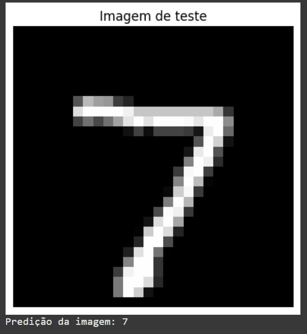
To visualize the image we want to classify:

sample_image, _ = testset[0]
plt.imshow(sample_image.squeeze(), cmap='gray')
plt.title("Test Image")
plt.axis("off")
plt.show()

Here, a test image is extracted from the testset and displayed.

• squeeze() removes extra dimensions, like the color channel.

• The image is displayed using matplotlib.

Finally, we perform inference on the displayed image and print the prediction:

prediction = inference(model, sample_image) 
print(f'Predicted image: {prediction}')

The inference is performed on the displayed image, and the prediction is printed in the terminal. We can see that our classifier has correctly identified the digit!

Next Steps

After training, our neural network achieved a reasonable accuracy (91.82%), but there is still room for improvement. To optimize performance, we can:

• Add more layers to the network (deep learning).

• Test different activation functions.

• Adjust hyperparameters, such as learning rate and number of epochs.

• Use techniques such as normalization and dropout.

We can also experiment with convolutional neural networks (CNNs).

For image classification problems, convolutional networks generally perform better. CNNs are especially good at capturing spatial patterns in images.

Feel free to explore other approaches that could further improve the model’s performance!

You can find the code on Colab at: https://exploringartificialintelligence.substack.com/p/notebooks

Conclusions

Our code trained a simple MLP neural network to classify images from the MNIST dataset, which contains images of handwritten digits in 28x28 pixels.

The training was done using a stochastic gradient descent (SGD) optimizer, and the loss function used was CrossEntropyLoss.

After training, the model was tested and evaluated in terms of accuracy. As we saw, the model performed reasonably, but it can still be improved in various ways.

If you are just starting with PyTorch, this is a great starting point. 😉

I hope you enjoyed the article!