
Random Forest: How to Improve Accuracy with Multiple Decision Trees
With Random Forest, each tree contributes to a more robust and accurate decision.


Hello!
Continuing the series "Top 8 Machine Learning Algorithms: Everything You Need to Know," today we’re going to explore Random Forest.
In the last post, we saw how decision trees offer an intuitive and visual way to make decisions based on data.
Now, imagine combining several decision trees to improve accuracy and avoid overfitting? This is possible with Random Forest, a powerful and versatile technique for classification and regression tasks.
But what exactly is Random Forest, how does it work, and why is it so widely used? Let's explore these questions in this article.
You can find the code on Colab at: https://exploringartificialintelligence.substack.com/p/notebooks
What is Random Forest?
Random Forest is a supervised learning algorithm based on a set of decision trees. It uses the concept of ensemble learning, where multiple models (in this case, decision trees) work together to achieve more accurate predictions.
Ensemble learning in Machine Learning is a technique that combines multiple models to improve the accuracy and robustness of predictions. Instead of relying on a single model, the ensemble uses the "wisdom of crowds," where combining multiple predictions from different models leads to stronger and more reliable performance.
Each tree in the forest gives a prediction, and Random Forest combines these predictions to make a final decision. For classification tasks, the final result is determined by majority voting; for regression, the average of the predictions is calculated.
How Does Random Forest Work?
Random Forest builds several decision trees in parallel, but with two key ingredients that introduce diversity and reduce the risk of overfitting:
Bootstrap Aggregation (Bagging): Instead of training all the trees on the same dataset, the algorithm selects random subsets of the training set with replacement. This means each tree is trained on a slightly different sample of the original data.
Random Feature Selection: During the training of each tree node, the algorithm randomly selects a subset of features (attributes or characteristics) rather than considering all available features. This prevents a single feature from dominating the decision-making process.
With these strategies, Random Forest combines the power of multiple individual trees to create a robust and accurate model.
Advantages of Random Forest
Robustness Against Overfitting: Due to the use of multiple trees and randomness, Random Forest is less prone to overfitting the model to the training data.
Accuracy: It often outperforms simpler algorithms, especially in problems with many features or noisy data.
Ease of Use: Random Forest requires minimal data preparation and can handle categorical and numerical data without the need for scaling.
Feature Importance: The algorithm provides a feature importance metric, allowing identification of which variables have the greatest impact on predictions.
Versatility: Works well for classification, regression, and even tasks like anomaly detection.
Disadvantages of Random Forest
Despite its advantages, Random Forest also presents some challenges:
Computational Complexity: Models with many trees can be computationally intensive and memory-hungry.
Reduced Interpretability: While individual trees are easy to interpret, the combination of hundreds or thousands of trees makes explaining the model challenging.
Practical Applications
Random Forest is widely used in fields such as:
Healthcare:
Medical diagnosis based on symptoms or lab tests.
Disease prediction based on genomic data.
Finance:
Credit scoring and fraud detection.
Asset price prediction.
E-commerce:
Product recommendation.
Churn analysis (customer attrition).
Environmental Science:
Natural disaster prediction.
Ecosystem modeling.
Natural Language Processing (NLP):
Text classification and sentiment analysis.
Practical Implementation in Python
Below is a simple example of how to use Random Forest with the scikit-learn library.
In this example, we'll use the Iris dataset, a classic dataset in machine learning, used for classification tasks. It contains 150 samples of flowers from the Iris species, with 4 features (sepal length and width, and petal length and width) for each sample, divided into three classes: setosa, versicolor, and virginica.

1 - Training
Create a new file in Jupyter Notebook and paste this code to load the dataset and perform the training:
from sklearn.ensemble import RandomForestClassifier
from sklearn.datasets import load_iris
from sklearn.model_selection import train_test_split
from sklearn.metrics import accuracy_score

# Load the Iris dataset
data = load_iris()
X = data.data  # Features
y = data.target  # Labels

# Split the data into training and testing sets
X_train, X_test, y_train, y_test = train_test_split(X, y, test_size=0.3, random_state=42)

# Create and train the model
model = RandomForestClassifier(n_estimators=100, random_state=42)
model.fit(X_train, y_train)

# Make predictions and evaluate the model
y_pred = model.predict(X_test)
accuracy = accuracy_score(y_test, y_pred)

print(f"Model accuracy: {accuracy:.2f}")
2 - Inference
Now, we can make inferences with the trained model. Let's assume we have two Iris flowers for which we want to determine the species. We will extract the sepal and petal length and width and send them to the model.
# New data for inference
new_data = [[5.1, 3.5, 1.4, 0.2],  # Example 1
            [6.7, 3.1, 4.7, 1.5]]  # Example 2

# Make the prediction
predictions = model.predict(new_data)

# Display the predictions
print("Predictions for the new data:", predictions)
Result:
Predictions for the new data: [0 1]Our model made predictions for the two new examples, and the predicted classes for these examples are 0 and 1, which correspond to the class indices in the dataset, namely setosa and versicolor.
3 - Visualizing Feature Importance
Now, let's see which features of the dataset are most important for the model.
import matplotlib.pyplot as plt
import numpy as np

# Get feature importance
importance = model.feature_importances_

# Create the feature importance plot
features = data.feature_names
indices = np.argsort(importance)

plt.figure(figsize=(8, 6))
plt.title("Feature Importance")
plt.barh(range(len(indices)), importance[indices], align="center")
plt.yticks(range(len(indices)), [features[i] for i in indices])
plt.xlabel("Importance")
plt.show()
Result:
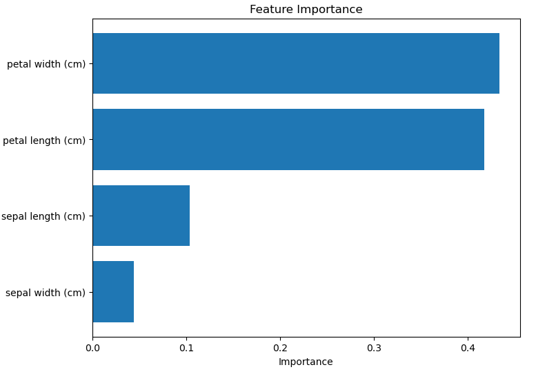
This chart shows the relative importance of each feature in the model. The y-axis contains the names of the variables (features), and the x-axis shows the importance of each one for the model's decisions.
4 - Confusion Matrix
The confusion matrix helps evaluate the model's performance by showing how correctly or incorrectly it classified the samples of each class.
from sklearn.metrics import confusion_matrix
import seaborn as sns

# Generate the confusion matrix
confusion_matrix_result = confusion_matrix(y_test, y_pred)

# Plot the confusion matrix
plt.figure(figsize=(8, 6))
sns.heatmap(confusion_matrix_result, annot=True, fmt="d", cmap="Blues", xticklabels=data.target_names, yticklabels=data.target_names)
plt.title("Confusion Matrix")
plt.xlabel("Prediction")
plt.ylabel("Actual")
plt.show()
Result:
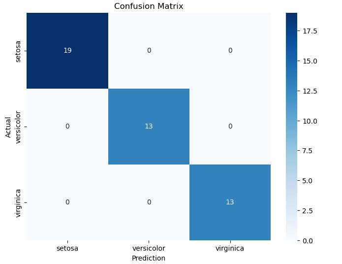
The confusion matrix shows the number of correct and incorrect predictions made by the model for each class. The diagonal cells indicate the correct predictions, while the off-diagonal cells show the errors.
Our matrix indicates excellent performance from the classification model, meaning the model achieved a 100% accuracy rate.
You can find the code on Colab at: https://exploringartificialintelligence.substack.com/p/notebooks
Conclusion
Random Forest is a powerful and flexible tool, widely used in various domains due to its robustness, accuracy, and ease of use. While it may not be perfect for all cases, it is an excellent starting point for many supervised learning problems.
If you're exploring the world of machine learning, it's worth experimenting with Random Forest and discovering how it can add value to your projects!
In the next post, we'll explore Support Vector Machines (SVM).
See you!! 🩷
Always a fresh new approach for AI. Thanks